Chapter 15 Mediation & Moderation
These notes are adapted from this tutorial: Mediation and moderation
15.1 Learning goals
- Understanding what controlling for variables means.
- Learning a graphical procedure that helps identify when it’s good vs. bad to control for variables.
- Simulating a mediation analysis.
- Baron and Kenny’s (1986) steps for mediation.
- Testing the significance of a mediation.
- Sobel test.
- Bootstrapping.
- Bayesian approach.
- Limitations of mediation analysis.
- Simulating a moderator effect.
15.2 Recommended reading
15.3 Load packages and set plotting theme
library("knitr")         # for knitting RMarkdown
library("kableExtra")    # for making nice tables
library("janitor")       # for cleaning column names
library("mediation")     # for mediation and moderation analysis
library("multilevel")    # Sobel test
library("broom")         # tidying up regression results
library("DiagrammeR")    # for drawing diagrams
library("DiagrammeRsvg") # for exporting pdfs of graphs
library("rsvg")          # for exporting pdfs of graphs
library("tidyverse") # for wrangling, plotting, etc. theme_set(theme_classic() + #set the theme
theme(text = element_text(size = 20))) #set the default text size
opts_chunk$set(comment = "",
fig.show = "hold")
options(dplyr.summarise.inform = FALSE) # Disable summarize ungroup messages15.4 Controlling for variables
15.4.1 Illustration of the d-separation algorithm
- Question: Are D and E independent?
15.4.1.1 Full DAG
g = grViz("
digraph neato {

  graph[layout = neato]

  # general settings for all nodes
  node [
    shape = circle,
    style = filled,
    color = black,
    label = ''
    fontname = 'Helvetica',
    fontsize = 16,
    fillcolor = lightblue
    ]

  # labels for each node
  a [label = 'A' pos = '0,0!']
  b [label = 'B'  pos = '2,0!']
  c [label = 'C' pos = '1,-1!']
  d [label = 'D' pos = '0,-2!']
  e [label = 'E' pos = '2,-2!']
  f [label = 'F' pos = '1,-3!']
  g [label = 'G' pos = '0,-4!']

  # edges between nodes
  edge [color = black]
  a -> c
  b -> c
  c -> {d e}
  d -> f
  f -> g

  # direction in which arrows are drawn (from left to right)
  rankdir = LR
}
")

# export as pdf
# g %>%
#   export_svg %>%
#   charToRaw %>%
#   rsvg_pdf("figures/dag.pdf")

# show plot
g
15.4.1.2 Draw the ancestral graph
g = grViz("
digraph neato {

  graph[layout = neato]

  # general settings for all nodes
  node [
    shape = circle,
    style = filled,
    color = black,
    label = ''
    fontname = 'Helvetica',
    fontsize = 16,
    fillcolor = lightblue
    ]

  # labels for each node
  a [label = 'A' pos = '0,0!']
  b [label = 'B'  pos = '2,0!']
  c [label = 'C' pos = '1,-1!']
  d [label = 'D' pos = '0,-2!']
  e [label = 'E' pos = '2,-2!']

  # edges between nodes
  edge [color = black]
  a -> c
  b -> c
  c -> {d e}

  # direction in which arrows are drawn (from left to right)
  rankdir = LR
}
")

# export as pdf
# g %>%
#   export_svg %>%
#   charToRaw %>%
#   rsvg_pdf("figures/ancestral_graph.pdf")

# show plot
g
15.4.1.3 “Moralize” the ancestral graph by “marrying” any parents, and disorient by replacing arrows with edges
g = grViz("
graph neato {

  graph[layout = neato]

  # general settings for all nodes
  node [
    shape = circle,
    style = filled,
    color = black,
    label = ''
    fontname = 'Helvetica',
    fontsize = 16,
    fillcolor = lightblue
    ]

  # labels for each node
  a [label = 'A' pos = '0,0!']
  b [label = 'B'  pos = '2,0!']
  c [label = 'C' pos = '1,-1!']
  d [label = 'D' pos = '0,-2!']
  e [label = 'E' pos = '2,-2!']

  # edges between nodes
  edge [color = black]
  a -- c
  b -- c
  c -- {d e}

  edge [color = black]
  a -- b

  # direction in which arrows are drawn (from left to right)
  rankdir = LR
}
")

# export as pdf
# g %>%
#   export_svg %>%
#   charToRaw %>%
#   rsvg_pdf("figures/moralize_and_disorient.pdf")

# show plot
g- For the case in which we check whether D and E are independent conditioned on C
g = grViz("
graph neato {

  graph[layout = neato]

  # general settings for all nodes
  node [
    shape = circle,
    style = filled,
    color = black,
    label = ''
    fontname = 'Helvetica',
    fontsize = 16,
    fillcolor = lightblue
    ]

  # labels for each node
  a [label = 'A' pos = '0,0!']
  b [label = 'B'  pos = '2,0!']
  d [label = 'D' pos = '0,-2!']
  e [label = 'E' pos = '2,-2!']

  # edges between nodes
  edge [color = black]

  edge [color = black]
  a -- b

  # direction in which arrows are drawn (from left to right)
  rankdir = LR
}
")

## export as pdf
#g %>%
#  export_svg %>%
#  charToRaw %>%
#  rsvg_pdf("figures/moralize_and_disorient2.pdf")

# show plot
g
15.4.2 Good controls
15.4.2.1 Common cause (with direct link between X and Y)
15.4.2.1.1 DAG
g = grViz("
digraph neato {

  graph[layout = neato]

  # general settings for all nodes
  node [
    shape = circle,
    style = filled,
    color = black,
    label = ''
    fontname = 'Helvetica',
    fontsize = 16,
    fillcolor = lightblue
    ]

  # labels for each node
  x [label = 'X' pos = '0,0!']
  y [label = 'Y'  pos = '2,0!']
  z [label = 'Z' pos = '1,1!', fontcolor = 'red']

  # edges between nodes
  edge [color = black]
  x -> y
  z -> {x y}

  # direction in which arrows are drawn (from left to right)
  rankdir = LR
}
")

# export as pdf
# g %>%
#   export_svg %>%
#   charToRaw %>%
#   rsvg_pdf("figures/common_cause1.pdf")

# show plot
g
15.4.2.1.2 Regression
set.seed(1)

n = 1000
b_zx = 2
b_xy = 2
b_zy = 2
sd = 1

fun_error = function(n, sd){
  rnorm(n = n,
        mean = 0,
        sd = sd)
}

df = tibble(z = fun_error(n, sd),
            x = b_zx * z + fun_error(n, sd),
            y = b_zy * z + b_xy * x + fun_error(n, sd))

# without control
lm(formula = y ~ x,
   data = df) %>%
  summary()
Call:
lm(formula = y ~ x, data = df)

Residuals:
    Min      1Q  Median      3Q     Max
-4.6011 -0.9270 -0.0506  0.9711  4.0454

Coefficients:
            Estimate Std. Error t value Pr(>|t|)
(Intercept)  0.02449    0.04389   0.558    0.577
x            2.82092    0.01890 149.225   <2e-16 ***
---
Signif. codes:  0 '***' 0.001 '**' 0.01 '*' 0.05 '.' 0.1 ' ' 1

Residual standard error: 1.388 on 998 degrees of freedom
Multiple R-squared:  0.9571,    Adjusted R-squared:  0.9571
F-statistic: 2.227e+04 on 1 and 998 DF,  p-value: < 2.2e-16
# with control
lm(formula = y ~ x + z,
data = df) %>%
summary()
Call:
lm(formula = y ~ x + z, data = df)

Residuals:
    Min      1Q  Median      3Q     Max
-3.6151 -0.6564 -0.0223  0.6815  2.8132

Coefficients:
            Estimate Std. Error t value Pr(>|t|)
(Intercept)  0.01624    0.03260   0.498    0.618
x            2.02202    0.03135  64.489   <2e-16 ***
z            2.00501    0.07036  28.497   <2e-16 ***
---
Signif. codes:  0 '***' 0.001 '**' 0.01 '*' 0.05 '.' 0.1 ' ' 1

Residual standard error: 1.031 on 997 degrees of freedom
Multiple R-squared:  0.9764,    Adjusted R-squared:  0.9763
F-statistic: 2.059e+04 on 2 and 997 DF,  p-value: < 2.2e-16
15.4.2.1.3 Moralize and disorient the ancestral graph
g = grViz("
graph neato {

  graph[layout = neato]

  # general settings for all nodes
  node [
    shape = circle,
    style = filled,
    color = black,
    label = ''
    fontname = 'Helvetica',
    fontsize = 16,
    fillcolor = lightblue
    ]

  # labels for each node
  x [label = 'X' pos = '0,0!']
  y [label = 'Y'  pos = '2,0!']
  z [label = 'Z' pos = '1,1!', fontcolor = 'red']

  # edges between nodes
  edge [color = black]
  x -- y
  z -- {x y}

  # direction in which arrows are drawn (from left to right)
  rankdir = LR
}
")

# export as pdf
# g %>%
#   export_svg %>%
#   charToRaw %>%
#   rsvg_pdf("figures/common_cause1_undirected.pdf")
#   # rsvg_pdf("figures/common_cause1_undirected2.pdf")

# show plot
g
15.4.2.2 Common cause (without direct link between X and Y)
15.4.2.2.1 DAG
g = grViz("
digraph neato {

  graph[layout = neato]

  # general settings for all nodes
  node [
    shape = circle,
    style = filled,
    color = black,
    label = ''
    fontname = 'Helvetica',
    fontsize = 16,
    fillcolor = lightblue
    ]

  # labels for each node
  x [label = 'X' pos = '0,0!']
  y [label = 'Y'  pos = '2,0!']
  z [label = 'Z' pos = '1,1!', fontcolor = 'red']

  # edges between nodes
  edge [color = black]
  z -> {x y}

  # direction in which arrows are drawn (from left to right)
  rankdir = LR
}
")

# export as pdf
# g %>%
#   export_svg %>%
#   charToRaw %>%
#   rsvg_pdf("figures/common_cause2.pdf")

# show plot
g
15.4.2.2.2 Regression
set.seed(1)
n = 1000
b_zx = 2
b_zy = 2
sd = 1

fun_error = function(n, sd){
  rnorm(n = n,
        mean = 0,
        sd = sd)
}

df = tibble(z = fun_error(n, sd),
            x = b_zx * z + fun_error(n, sd),
            y = b_zy * z + fun_error(n, sd))

# without control
lm(formula = y ~ x,
   data = df) %>%
  summary()
Call:
lm(formula = y ~ x, data = df)

Residuals:
    Min      1Q  Median      3Q     Max
-4.6011 -0.9270 -0.0506  0.9711  4.0454

Coefficients:
            Estimate Std. Error t value Pr(>|t|)
(Intercept)  0.02449    0.04389   0.558    0.577
x            0.82092    0.01890  43.426   <2e-16 ***
---
Signif. codes:  0 '***' 0.001 '**' 0.01 '*' 0.05 '.' 0.1 ' ' 1

Residual standard error: 1.388 on 998 degrees of freedom
Multiple R-squared:  0.6539,    Adjusted R-squared:  0.6536
F-statistic:  1886 on 1 and 998 DF,  p-value: < 2.2e-16
# with control
lm(formula = y ~ x + z,
data = df) %>%
summary()
Call:
lm(formula = y ~ x + z, data = df)

Residuals:
    Min      1Q  Median      3Q     Max
-3.6151 -0.6564 -0.0223  0.6815  2.8132

Coefficients:
            Estimate Std. Error t value Pr(>|t|)
(Intercept)  0.01624    0.03260   0.498    0.618
x            0.02202    0.03135   0.702    0.483
z            2.00501    0.07036  28.497   <2e-16 ***
---
Signif. codes:  0 '***' 0.001 '**' 0.01 '*' 0.05 '.' 0.1 ' ' 1

Residual standard error: 1.031 on 997 degrees of freedom
Multiple R-squared:  0.8093,    Adjusted R-squared:  0.8089
F-statistic:  2115 on 2 and 997 DF,  p-value: < 2.2e-16
15.4.3 Bad controls
15.4.3.1 Common effect
15.4.3.1.1 DAG
g = grViz("
digraph neato {

  graph[layout = neato]

  # general settings for all nodes
  node [
    shape = circle,
    style = filled,
    color = black,
    label = ''
    fontname = 'Helvetica',
    fontsize = 16,
    fillcolor = lightblue
    ]

  # labels for each node
  x [label = 'X' pos = '0,0!']
  y [label = 'Y'  pos = '2,0!']
  z [label = 'Z' pos = '1,-1!', fontcolor = 'red']

  # edges between nodes
  edge [color = black]
  x -> z
  y -> z

  # direction in which arrows are drawn (from left to right)
  rankdir = LR
}
")

# export as pdf
# g %>%
#   export_svg %>%
#   charToRaw %>%
#   rsvg_pdf("figures/common_effect.pdf")

# show plot
g
15.4.3.1.2 Regression
set.seed(1)
n = 1000
b_xz = 2
b_yz = 2
sd = 1

fun_error = function(n, sd){
  rnorm(n = n,
        mean = 0,
        sd = sd)
}

df = tibble(x = fun_error(n, sd),
            y = fun_error(n, sd),
            z = x * b_xz + y * b_yz + fun_error(n, sd))

# without control
lm(formula = y ~ x,
   data = df) %>%
  summary()
Call:
lm(formula = y ~ x, data = df)

Residuals:
    Min      1Q  Median      3Q     Max
-3.2484 -0.6720 -0.0138  0.7554  3.6443

Coefficients:
             Estimate Std. Error t value Pr(>|t|)
(Intercept) -0.016187   0.032905  -0.492    0.623
x            0.006433   0.031809   0.202    0.840

Residual standard error: 1.04 on 998 degrees of freedom
Multiple R-squared:  4.098e-05, Adjusted R-squared:  -0.000961
F-statistic: 0.0409 on 1 and 998 DF,  p-value: 0.8398
# with control
lm(formula = y ~ x + z,
data = df) %>%
summary()
Call:
lm(formula = y ~ x + z, data = df)

Residuals:
     Min       1Q   Median       3Q      Max
-1.35547 -0.30016  0.00298  0.31119  1.73408

Coefficients:
             Estimate Std. Error t value Pr(>|t|)
(Intercept) -0.009608   0.014477  -0.664    0.507
x           -0.816164   0.018936 -43.102   <2e-16 ***
z            0.398921   0.006186  64.489   <2e-16 ***
---
Signif. codes:  0 '***' 0.001 '**' 0.01 '*' 0.05 '.' 0.1 ' ' 1

Residual standard error: 0.4578 on 997 degrees of freedom
Multiple R-squared:  0.8066,    Adjusted R-squared:  0.8062
F-statistic:  2079 on 2 and 997 DF,  p-value: < 2.2e-16
15.4.3.1.3 Moralize and disorient the ancestral graph
g = grViz("
graph neato {

  graph[layout = neato]

  # general settings for all nodes
  node [
    shape = circle,
    style = filled,
    color = black,
    label = ''
    fontname = 'Helvetica',
    fontsize = 16,
    fillcolor = lightblue
    ]

  # labels for each node
  x [label = 'X' pos = '0,0!']
  y [label = 'Y'  pos = '2,0!']
  z [label = 'Z' pos = '1,-1!', fontcolor = 'red']

  # edges between nodes
  edge [color = black]
  x -- y
  x -- z
  y -- z

  # direction in which arrows are drawn (from left to right)
  rankdir = LR
}
")

# export as pdf
# g %>%
#   export_svg %>%
#   charToRaw %>%
#   rsvg_pdf("figures/common_effect_undirected1.pdf")
#   rsvg_pdf("figures/common_effect_undirected2.pdf")

# show plot
g
15.4.3.2 Causal chain 1
15.4.3.2.1 DAG
g = grViz("
digraph neato {

  graph[layout = neato]

  # general settings for all nodes
  node [
    shape = circle,
    style = filled,
    color = black,
    label = ''
    fontname = 'Helvetica',
    fontsize = 16,
    fillcolor = lightblue
    ]

  # labels for each node
  x [label = 'X' pos = '0,0!']
  y [label = 'Y'  pos = '2,0!']
  z [label = 'Z' pos = '1, 0!', fontcolor = 'red']

  # edges between nodes
  edge [color = black]
  x -> z
  z -> y

  # direction in which arrows are drawn (from left to right)
  rankdir = LR
}
")

# # export as pdf
# g %>%
#   export_svg %>%
#   charToRaw %>%
#   rsvg_pdf("figures/causal_chain.pdf")

# show plot
g
15.4.3.2.2 Regression
set.seed(1)
n = 20
b_xz = 2
b_zy = 2
sd = 1

fun_error = function(n, sd){
  rnorm(n = n,
        mean = 0,
        sd = sd)
}

df = tibble(x = fun_error(n, sd),
            z = x * b_xz + fun_error(n, sd),
            y = z * b_zy + fun_error(n, sd))

# without control
lm(formula = y ~ x,
   data = df) %>%
  summary()
Call:
lm(formula = y ~ x, data = df)

Residuals:
   Min     1Q Median     3Q    Max
-3.336 -1.208  0.209  1.220  3.189

Coefficients:
            Estimate Std. Error t value Pr(>|t|)
(Intercept)   0.1547     0.3982   0.388    0.702
x             3.8488     0.4374   8.799 6.15e-08 ***
---
Signif. codes:  0 '***' 0.001 '**' 0.01 '*' 0.05 '.' 0.1 ' ' 1

Residual standard error: 1.741 on 18 degrees of freedom
Multiple R-squared:  0.8114,    Adjusted R-squared:  0.8009
F-statistic: 77.43 on 1 and 18 DF,  p-value: 6.154e-08
# with control
lm(formula = y ~ x + z,
data = df) %>%
summary()
Call:
lm(formula = y ~ x + z, data = df)

Residuals:
     Min       1Q   Median       3Q      Max
-1.35959 -0.56643 -0.06193  0.48088  1.80592

Coefficients:
            Estimate Std. Error t value Pr(>|t|)
(Intercept)  0.09559    0.18177   0.526    0.606
x            0.64724    0.43278   1.496    0.153
z            1.78614    0.21425   8.337 2.07e-07 ***
---
Signif. codes:  0 '***' 0.001 '**' 0.01 '*' 0.05 '.' 0.1 ' ' 1

Residual standard error: 0.7943 on 17 degrees of freedom
Multiple R-squared:  0.9629,    Adjusted R-squared:  0.9586
F-statistic: 220.8 on 2 and 17 DF,  p-value: 6.868e-13
15.4.3.3 Causal chain 2
15.4.3.3.1 DAG
g = grViz("
digraph neato {

  graph[layout = neato]

  # general settings for all nodes
  node [
    shape = circle,
    style = filled,
    color = black,
    label = ''
    fontname = 'Helvetica',
    fontsize = 16,
    fillcolor = lightblue
    ]

  # labels for each node
  x [label = 'X' pos = '0,0!']
  y [label = 'Y'  pos = '1,0!']
  z [label = 'Z' pos = '2, 0!', fontcolor = 'red']

  # edges between nodes
  edge [color = black]
  x -> y
  y -> z

  # direction in which arrows are drawn (from left to right)
  rankdir = LR
}
")

# # export as pdf
# g %>%
#   export_svg %>%
#   charToRaw %>%
#   rsvg_pdf("figures/causal_chain2.pdf")

# show plot
g
15.4.3.3.2 Regression
set.seed(1)
n = 20
b_xy = 2
b_yz = 2
sd = 1

fun_error = function(n, sd){
  rnorm(n = n,
        mean = 0,
        sd = sd)
}

df = tibble(x = fun_error(n, sd),
            y = x * b_xy + fun_error(n, sd),
            z = y * b_yz + fun_error(n, sd),)

# without control
lm(formula = y ~ x,
   data = df) %>%
  summary()
Call:
lm(formula = y ~ x, data = df)

Residuals:
     Min       1Q   Median       3Q      Max
-1.69133 -0.43739 -0.07132  0.68033  1.63937

Coefficients:
            Estimate Std. Error t value Pr(>|t|)
(Intercept)  0.03307    0.19981   0.166     0.87
x            1.79245    0.21951   8.166 1.83e-07 ***
---
Signif. codes:  0 '***' 0.001 '**' 0.01 '*' 0.05 '.' 0.1 ' ' 1

Residual standard error: 0.8738 on 18 degrees of freedom
Multiple R-squared:  0.7874,    Adjusted R-squared:  0.7756
F-statistic: 66.68 on 1 and 18 DF,  p-value: 1.827e-07
# with control
lm(formula = y ~ x + z,
data = df) %>%
summary()
Call:
lm(formula = y ~ x + z, data = df)

Residuals:
    Min      1Q  Median      3Q     Max
-0.9023 -0.2316  0.1173  0.2396  0.6319

Coefficients:
            Estimate Std. Error t value Pr(>|t|)
(Intercept) -0.03650    0.09153  -0.399    0.695
x            0.06113    0.23056   0.265    0.794
z            0.44983    0.05396   8.337 2.07e-07 ***
---
Signif. codes:  0 '***' 0.001 '**' 0.01 '*' 0.05 '.' 0.1 ' ' 1

Residual standard error: 0.3986 on 17 degrees of freedom
Multiple R-squared:  0.9582,    Adjusted R-squared:  0.9533
F-statistic:   195 on 2 and 17 DF,  p-value: 1.896e-12
15.4.3.4 Bias amplification
15.4.3.4.1 DAG
g = grViz("
digraph neato {

  graph[layout = neato]

  # general settings for all nodes
  node [
    shape = circle,
    style = filled,
    color = black,
    label = ''
    fontname = 'Helvetica',
    fontsize = 16,
    fillcolor = lightblue
    ]

  # labels for each node
  x [label = 'X' pos = '0,0!']
  y [label = 'Y'  pos = '2,0!']
  z [label = 'Z' pos = '-1, 1!', fontcolor = 'red']
  u [label = 'U' pos = '1, 1!', fillcolor = 'white']

  # edges between nodes
  edge [color = black]
  x -> y
  z -> x
  u -> {x y}

  # direction in which arrows are drawn (from left to right)
  rankdir = LR
}
")

# # export as pdf
# g %>%
#   export_svg %>%
#   charToRaw %>%
#   rsvg_pdf("figures/bias_amplification.pdf")

# show plot
g
15.4.3.5 Regression
set.seed(1)
n = 20
b_xy = 2
b_ux = 2
b_uy = 2
b_zx = 2
sd = 1

fun_error = function(n, sd){
  rnorm(n = n,
        mean = 0,
        sd = sd)
}

df = tibble(u = fun_error(n, sd),
            z = fun_error(n, sd),
            x = u * b_ux + z * b_zx + fun_error(n, sd),
            y = u * b_uy + x * b_xy + fun_error(n, sd))

# without control
lm(formula = y ~ x,
   data = df) %>%
  summary()
Call:
lm(formula = y ~ x, data = df)

Residuals:
    Min      1Q  Median      3Q     Max
-2.2838 -0.8662 -0.2281  0.7201  3.1619

Coefficients:
            Estimate Std. Error t value Pr(>|t|)
(Intercept)   0.1903     0.3282    0.58    0.569
x             2.5771     0.1375   18.74 2.96e-13 ***
---
Signif. codes:  0 '***' 0.001 '**' 0.01 '*' 0.05 '.' 0.1 ' ' 1

Residual standard error: 1.434 on 18 degrees of freedom
Multiple R-squared:  0.9512,    Adjusted R-squared:  0.9485
F-statistic: 351.1 on 1 and 18 DF,  p-value: 2.961e-13
# with control
lm(formula = y ~ x + z,
data = df) %>%
summary()
Call:
lm(formula = y ~ x + z, data = df)

Residuals:
    Min      1Q  Median      3Q     Max
-1.9114 -0.4876 -0.1044  0.6333  1.8935

Coefficients:
            Estimate Std. Error t value Pr(>|t|)
(Intercept)  0.07431    0.24564   0.303  0.76594
x            2.78984    0.11553  24.147 1.35e-14 ***
z           -1.25270    0.31719  -3.949  0.00103 **
---
Signif. codes:  0 '***' 0.001 '**' 0.01 '*' 0.05 '.' 0.1 ' ' 1

Residual standard error: 1.066 on 17 degrees of freedom
Multiple R-squared:  0.9746,    Adjusted R-squared:  0.9716
F-statistic: 325.7 on 2 and 17 DF,  p-value: 2.793e-14
15.5 Mediation
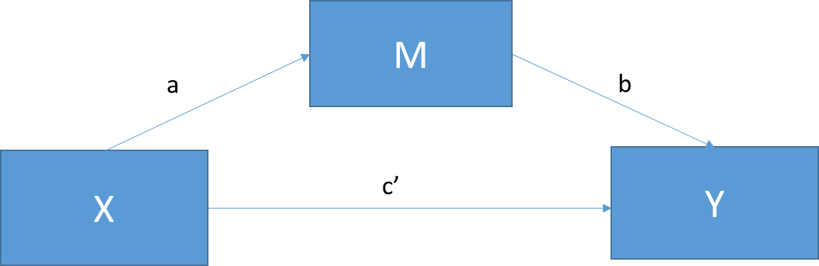
Figure 15.1: Basic mediation model. c = the total effect of X on Y; c = c’ + ab; c’ = the direct effect of X on Y after controlling for M; c’ = c - ab; ab = indirect effect of X on Y.
Mediation tests whether the effects of X (the independent variable) on Y (the dependent variable) operate through a third variable, M (the mediator). In this way, mediators explain the causal relationship between two variables or “how” the relationship works, making it a very popular method in psychological research.
Figure 15.1 shows the standard mediation model. Perfect mediation occurs when the effect of X on Y decreases to 0 with M in the model. Partial mediation occurs when the effect of X on Y decreases by a nontrivial amount (the actual amount is up for debate) with M in the model.
Important: Both mediation and moderation assume that the DV did not CAUSE the mediator/moderator.
15.5.1 Generate data
# make example reproducible
set.seed(123)

# number of participants
n = 100

# generate data
df.mediation = tibble(x = rnorm(n, 75, 7), # grades
  m = 0.7 * x + rnorm(n, 0, 5), # self-esteem
  y = 0.4 * m + rnorm(n, 0, 5)) # happiness
15.5.2 Method 1: Baron & Kenny’s (1986) indirect effect method
The Baron and Kenny (1986) method is among the original methods for testing for mediation but tends to have low statistical power. It is covered in this chapter because it provides a very clear approach to establishing relationships between variables and is still occassionally requested by reviewers.
The three steps:
Estimate the relationship between \(X\) and \(Y\) (hours since dawn on degree of wakefulness). Path “c” must be significantly different from 0; must have a total effect between the IV & DV.
Estimate the relationship between \(X\) and \(M\) (hours since dawn on coffee consumption). Path “a” must be significantly different from 0; IV and mediator must be related.
Estimate the relationship between \(M\) and \(Y\) controlling for \(X\) (coffee consumption on wakefulness, controlling for hours since dawn). Path “b” must be significantly different from 0; mediator and DV must be related. The effect of \(X\) on \(Y\) decreases with the inclusion of \(M\) in the model.
15.5.2.1 Total effect
Total effect of X on Y (not controlling for M).
# fit the model
fit.y_x = lm(formula = y ~ 1 + x,
            data = df.mediation)

# summarize the results
fit.y_x %>% summary()
Call:
lm(formula = y ~ 1 + x, data = df.mediation)

Residuals:
    Min      1Q  Median      3Q     Max
-10.917  -3.738  -0.259   2.910  12.540

Coefficients:
            Estimate Std. Error t value Pr(>|t|)
(Intercept)  8.78300    6.16002   1.426   0.1571
x            0.16899    0.08116   2.082   0.0399 *
---
Signif. codes:  0 '***' 0.001 '**' 0.01 '*' 0.05 '.' 0.1 ' ' 1

Residual standard error: 5.16 on 98 degrees of freedom
Multiple R-squared:  0.04237,   Adjusted R-squared:  0.0326
F-statistic: 4.336 on 1 and 98 DF,  p-value: 0.03993
15.5.2.2 Path a
fit.m_x = lm(formula = m ~ 1 + x,
            data = df.mediation)

fit.m_x %>% summary()
Call:
lm(formula = m ~ 1 + x, data = df.mediation)

Residuals:
    Min      1Q  Median      3Q     Max
-9.5367 -3.4175 -0.4375  2.9032 16.4520

Coefficients:
            Estimate Std. Error t value Pr(>|t|)
(Intercept)  2.29696    5.79432   0.396    0.693
x            0.66252    0.07634   8.678 8.87e-14 ***
---
Signif. codes:  0 '***' 0.001 '**' 0.01 '*' 0.05 '.' 0.1 ' ' 1

Residual standard error: 4.854 on 98 degrees of freedom
Multiple R-squared:  0.4346,    Adjusted R-squared:  0.4288
F-statistic: 75.31 on 1 and 98 DF,  p-value: 8.872e-14
15.5.2.3 Path b and c’
Effect of M on Y controlling for X.
fit.y_mx = lm(formula = y ~ 1 + m + x,
            data = df.mediation)

fit.y_mx %>% summary()
Call:
lm(formula = y ~ 1 + m + x, data = df.mediation)

Residuals:
    Min      1Q  Median      3Q     Max
-9.3651 -3.3037 -0.6222  3.1068 10.3991

Coefficients:
            Estimate Std. Error t value Pr(>|t|)
(Intercept)  7.80952    5.68297   1.374    0.173
m            0.42381    0.09899   4.281 4.37e-05 ***
x           -0.11179    0.09949  -1.124    0.264
---
Signif. codes:  0 '***' 0.001 '**' 0.01 '*' 0.05 '.' 0.1 ' ' 1

Residual standard error: 4.756 on 97 degrees of freedom
Multiple R-squared:  0.1946,    Adjusted R-squared:  0.1779
F-statistic: 11.72 on 2 and 97 DF,  p-value: 2.771e-05
15.5.2.4 Interpretation
fit.y_x %>%
  tidy() %>%
  mutate(path = "c") %>%
  bind_rows(fit.m_x %>%
              tidy() %>%
              mutate(path = "a"),
            fit.y_mx %>%
              tidy() %>%
              mutate(path = c("(Intercept)", "b", "c'"))) %>%
  filter(term != "(Intercept)") %>%
  mutate(significance = p.value < .05,
         dv = ifelse(path %in% c("c'", "b"), "y", "m")) %>%
  select(path, iv = term, dv, estimate, p.value, significance)
# A tibble: 4 x 6
path iv dv estimate p.value significance
<chr> <chr> <chr> <dbl> <dbl> <lgl>
1 c x m 0.169 3.99e- 2 TRUE
2 a x m 0.663 8.87e-14 TRUE
3 b m y 0.424 4.37e- 5 TRUE
4 c' x y -0.112 2.64e- 1 FALSE Here we find that our total effect model shows a significant positive relationship between hours since dawn (X) and wakefulness (Y). Our Path A model shows that hours since down (X) is also positively related to coffee consumption (M). Our Path B model then shows that coffee consumption (M) positively predicts wakefulness (Y) when controlling for hours since dawn (X).
Since the relationship between hours since dawn and wakefulness is no longer significant when controlling for coffee consumption, this suggests that coffee consumption does in fact mediate this relationship. However, this method alone does not allow for a formal test of the indirect effect so we don’t know if the change in this relationship is truly meaningful.
15.5.3 Method 2: Sobel Test
The Sobel Test tests whether the indirect effect from X via M to Y is significant.
# run the sobel test
fit.sobel = sobel(pred = df.mediation$x,
                  med = df.mediation$m,
                  out = df.mediation$y)

# calculate the p-value
(1 - pnorm(fit.sobel$z.value))*2
[1] 0.0001233403The relationship between “hours since dawn” and “wakefulness” is significantly mediated by “coffee consumption.”
The Sobel Test is largely considered an outdated method since it assumes that the indirect effect (ab) is normally distributed and tends to only have adequate power with large sample sizes. Thus, again, it is highly recommended to use the mediation bootstrapping method instead.
15.5.4 Method 3: Bootstrapping
The “mediation” packages uses the more recent bootstrapping method of Preacher and Hayes (2004) to address the power limitations of the Sobel Test.
This method does not require that the data are normally distributed, and is particularly suitable for small sample sizes.
library("mediation")

# bootstrapped mediation
fit.mediation = mediate(model.m = fit.m_x,
                        model.y = fit.y_mx,
                        treat = "x",
                        mediator = "m",
                        boot = T)
Running nonparametric bootstrap# summarize results
fit.mediation %>% summary()
Causal Mediation Analysis

Nonparametric Bootstrap Confidence Intervals with the Percentile Method

               Estimate 95% CI Lower 95% CI Upper p-value
ACME            0.28078      0.14133         0.43  <2e-16 ***
ADE            -0.11179     -0.30293         0.11   0.274
Total Effect    0.16899     -0.00539         0.35   0.056 .
Prop. Mediated  1.66151     -1.91644        10.16   0.056 .
---
Signif. codes:  0 '***' 0.001 '**' 0.01 '*' 0.05 '.' 0.1 ' ' 1

Sample Size Used: 100


Simulations: 1000 - ACME = Average causal mediation effect
- ADE = Average direct effect
- Total effect = ACME + ADE
Plot the results:
fit.mediation %>% plot()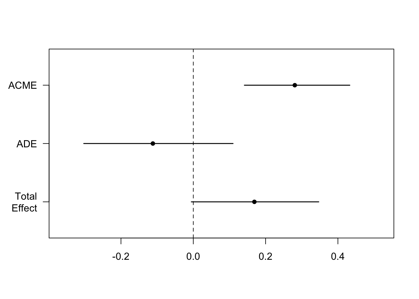
15.5.4.1 Interpretation
The mediate() function gives us our Average Causal Mediation Effects (ACME), our Average Direct Effects (ADE), our combined indirect and direct effects (Total Effect), and the ratio of these estimates (Prop. Mediated). The ACME here is the indirect effect of M (total effect - direct effect) and thus this value tells us if our mediation effect is significant.
15.6 Moderation
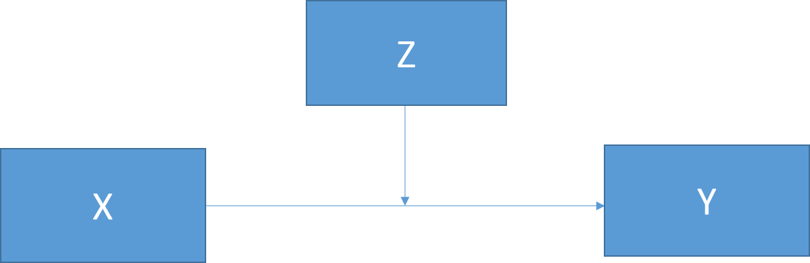
Figure 15.2: Basic moderation model.
Moderation can be tested by looking for significant interactions between the moderating variable (Z) and the IV (X). Notably, it is important to mean center both your moderator and your IV to reduce multicolinearity and make interpretation easier.
15.6.1 Generate data
# make example reproducible
set.seed(123)

# number of participants
n  = 100

df.moderation = tibble(x  = abs(rnorm(n, 6, 4)), # hours of sleep
                       x1 = abs(rnorm(n, 60, 30)), # adding some systematic variance to our DV
                       z  = rnorm(n, 30, 8), # ounces of coffee consumed
                       y  = abs((-0.8 * x) * (0.2 * z) - 0.5 * x - 0.4 * x1 + 10 +
                                  rnorm(n, 0, 3))) # attention Paid
15.6.2 Moderation analysis
# scale the predictors
df.moderation = df.moderation %>%
  mutate_at(vars(x, z), ~ scale(.)[,])

# run regression model with interaction
fit.moderation = lm(formula = y ~ 1 + x * z,
                    data = df.moderation)

# summarize result
fit.moderation %>%
  summary()
Call:
lm(formula = y ~ 1 + x * z, data = df.moderation)

Residuals:
    Min      1Q  Median      3Q     Max
-21.466  -8.972  -0.233   6.180  38.051

Coefficients:
            Estimate Std. Error t value Pr(>|t|)
(Intercept)   48.544      1.173  41.390  < 2e-16 ***
x             17.863      1.196  14.936  < 2e-16 ***
z              8.393      1.181   7.108 2.08e-10 ***
x:z            6.094      1.077   5.656 1.59e-07 ***
---
Signif. codes:  0 '***' 0.001 '**' 0.01 '*' 0.05 '.' 0.1 ' ' 1

Residual standard error: 11.65 on 96 degrees of freedom
Multiple R-squared:  0.7661,    Adjusted R-squared:  0.7587
F-statistic: 104.8 on 3 and 96 DF,  p-value: < 2.2e-16
15.6.2.1 Visualize result
# generate data grid with three levels of the moderator
df.newdata = df.moderation %>%
  expand(x = c(min(x),
               max(x)),
         z = c(mean(z) - sd(z),
               mean(z),
               mean(z) + sd(z))) %>%
  mutate(moderator = rep(c("low", "average", "high"), nrow(.)/3))

# predictions for the three levels of the moderator
df.prediction = fit.moderation %>%
  augment(newdata = df.newdata) %>%
  mutate(moderator = factor(moderator, levels = c("high", "average", "low")))

# visualize the result
df.moderation %>%
  ggplot(aes(x = x,
             y = y)) +
  geom_point() +
  geom_line(data = df.prediction,
            mapping = aes(y = .fitted,
                          group = moderator,
                          color = moderator),
            size = 1) +
  labs(x = "hours of sleep (z-scored)",
       y = "attention paid",
       color = "coffee consumed") +
  scale_color_brewer(palette = "Set1")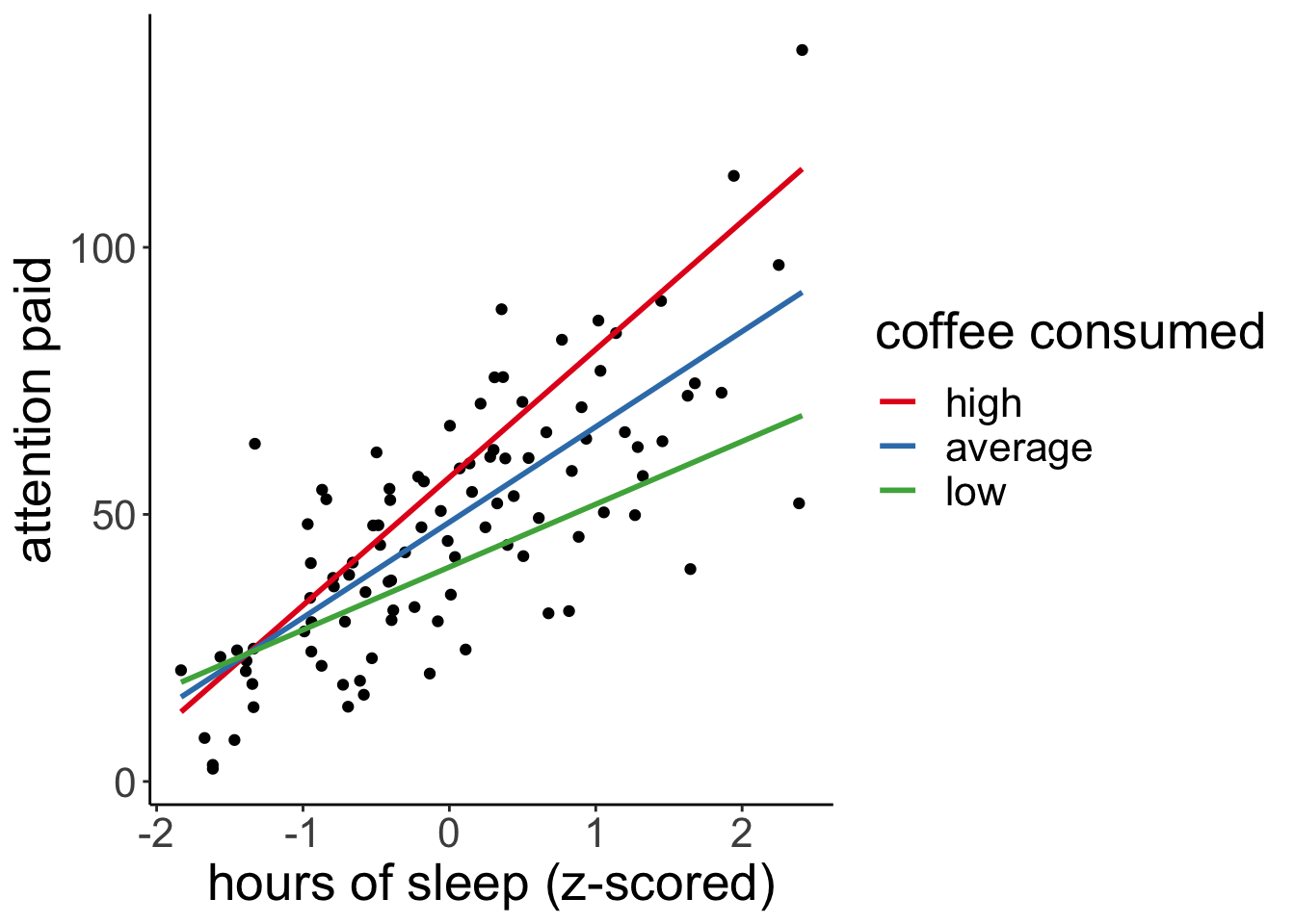
df.prediction %>%
  head(9) %>%
  kable(digits = 2) %>%
  kable_styling(bootstrap_options = "striped",
full_width = F)| x | z | moderator | .fitted |
|---|---|---|---|
| -1.83 | -1 | low | 18.58 |
| -1.83 | 0 | average | 15.80 |
| -1.83 | 1 | high | 13.02 |
| 2.41 | -1 | low | 68.52 |
| 2.41 | 0 | average | 91.60 |
| 2.41 | 1 | high | 114.68 |
15.7 Additional resources
15.7.1 Books
15.7.2 Tutorials
15.8 Session info
Information about this R session including which version of R was used, and what packages were loaded.
sessionInfo()R version 4.0.3 (2020-10-10)
Platform: x86_64-apple-darwin17.0 (64-bit)
Running under: macOS Catalina 10.15.7
Matrix products: default
BLAS: /Library/Frameworks/R.framework/Versions/4.0/Resources/lib/libRblas.dylib
LAPACK: /Library/Frameworks/R.framework/Versions/4.0/Resources/lib/libRlapack.dylib
locale:
[1] en_US.UTF-8/en_US.UTF-8/en_US.UTF-8/C/en_US.UTF-8/en_US.UTF-8
attached base packages:
[1] stats graphics grDevices utils datasets methods base
other attached packages:
[1] forcats_0.5.1 stringr_1.4.0 dplyr_1.0.4 purrr_0.3.4
[5] readr_1.4.0 tidyr_1.1.2 tibble_3.0.6 ggplot2_3.3.3
[9] tidyverse_1.3.0 rsvg_2.1 DiagrammeRsvg_0.1 DiagrammeR_1.0.6.1
[13] broom_0.7.3 multilevel_2.6 nlme_3.1-151 mediation_4.5.0
[17] sandwich_3.0-0 mvtnorm_1.1-1 Matrix_1.3-2 MASS_7.3-53
[21] janitor_2.1.0 kableExtra_1.3.1 knitr_1.31
loaded via a namespace (and not attached):
[1] fs_1.5.0 lubridate_1.7.9.2 webshot_0.5.2
[4] RColorBrewer_1.1-2 httr_1.4.2 tools_4.0.3
[7] backports_1.2.1 utf8_1.1.4 R6_2.5.0
[10] rpart_4.1-15 Hmisc_4.4-2 DBI_1.1.1
[13] colorspace_2.0-0 nnet_7.3-15 withr_2.4.1
[16] tidyselect_1.1.0 gridExtra_2.3 curl_4.3
[19] compiler_4.0.3 cli_2.3.0 rvest_0.3.6
[22] htmlTable_2.1.0 xml2_1.3.2 labeling_0.4.2
[25] bookdown_0.21 scales_1.1.1 checkmate_2.0.0
[28] digest_0.6.27 foreign_0.8-81 minqa_1.2.4
[31] rmarkdown_2.6 base64enc_0.1-3 jpeg_0.1-8.1
[34] pkgconfig_2.0.3 htmltools_0.5.1.1 lme4_1.1-26
[37] highr_0.8 dbplyr_2.0.0 readxl_1.3.1
[40] htmlwidgets_1.5.3 rlang_0.4.10 rstudioapi_0.13
[43] farver_2.1.0 visNetwork_2.0.9 generics_0.1.0
[46] zoo_1.8-8 jsonlite_1.7.2 magrittr_2.0.1
[49] Formula_1.2-4 fansi_0.4.2 Rcpp_1.0.6
[52] munsell_0.5.0 lifecycle_1.0.0 stringi_1.5.3
[55] yaml_2.2.1 snakecase_0.11.0 grid_4.0.3
[58] crayon_1.4.1 lattice_0.20-41 haven_2.3.1
[61] splines_4.0.3 hms_1.0.0 ps_1.6.0
[64] pillar_1.4.7 boot_1.3-26 lpSolve_5.6.15
[67] reprex_1.0.0 glue_1.4.2 evaluate_0.14
[70] V8_3.4.0 latticeExtra_0.6-29 data.table_1.13.6
[73] modelr_0.1.8 png_0.1-7 vctrs_0.3.6
[76] nloptr_1.2.2.2 cellranger_1.1.0 gtable_0.3.0
[79] assertthat_0.2.1 xfun_0.21 survival_3.2-7
[82] viridisLite_0.3.0 cluster_2.1.0 statmod_1.4.35
[85] ellipsis_0.3.1