Chapter 26 Reporting statistics
In this chapter, I’ll give a few examples for how to report statistical analysis.
26.1 General advice
Here is some general advice first:
- Make good figures!
- Use statistical models to answer concrete research questions.
- Illustrate the uncertainty in your statistical inferences.
- Report effect sizes.
26.1.1 Make good figures!
Chapters 2 and 3 go into how to make figures and also talk a little bit about what makes for a good figure. Personally, I like it when the figures give me a good sense for the actual data. For example, for an experimental study, I would like to get a good sense for the responses that participants gave in the different experimental conditions.
Sometimes, papers just report the results of statistical tests, or only visually display estimates of the parameters in the model. I’m not a fan of that since, as we’ve learned, the parameters of the model are only useful in so far the model captures the data-generating process reasonably well.
26.1.2 Use statistical models to answer concrete research questions.
Ideally, we formulate our research questions as statistical models upfront and pre-register our planned analyses (e.g. as an RMarkdown script with a complete analysis based on simulated data). We can then organize the results section by going through the sequence of research questions. Each statistical analysis then provides an answer to a specific research question.
26.1.3 Illustrate the uncertainty in your statistical inferences.
For frequentist statistics, we can calculate confidence intervals (e.g. using bootstrapping) and we should provide these intervals together with the point estimates of the model’s predictors.
For Bayesian statistics, we can calculate credible intervals based on the posterior over the model parameters.
Our figures should also indicate the uncertainty that we have in our statistical inferences (e.g. by adding confidence bands, or by showing some samples from the posterior).
26.1.4 Report effect sizes.
Rather than just saying whether the results of a statistical test was significant or not, you should, where possible, provide a measure of the effect size. Chapter 15 gives an overview of commonly used measures of effect size.
26.1.5 Reporting statistical results using RMarkdown
For reporting statistical results in RMarkdown, I recommend the papaja package (see this chapter in the online book).
26.2 Some concrete example
In this section, I’ll give a few concrete examples for how to report the results of statistical tests. Each example tries to implement the general advice mentioned above. I will discuss frequentist and Bayesian statistics separately.
26.2.1 Frequentist statistics
26.2.1.1 Simple regression
Research question: Do people with more income have a higher credit card balance?
ggplot(data = df.credit,
       mapping = aes(x = income,
                     y = balance)) +
  geom_smooth(method = "lm",
              color = "black") +
  geom_point(alpha = 0.2) +
  coord_cartesian(xlim = c(0, max(df.credit$income))) +
  labs(x = "Income in $1K per year",
       y = "Credit card balance in $")
## `geom_smooth()` using formula = 'y ~ x'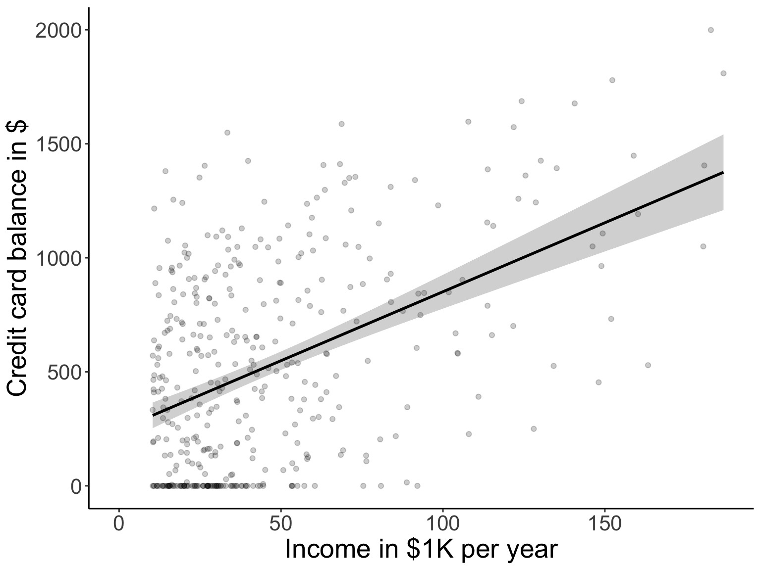
Figure 26.1: Relationship between income level and credit card balance. The error band indicates a 95% confidence interval.
##
## Call:
## lm(formula = balance ~ income, data = df.credit)
##
## Residuals:
##     Min      1Q  Median      3Q     Max
## -803.64 -348.99  -54.42  331.75 1100.25
##
## Coefficients:
##             Estimate Std. Error t value Pr(>|t|)
## (Intercept) 246.5148    33.1993   7.425  6.9e-13 ***
## income        6.0484     0.5794  10.440  < 2e-16 ***
## ---
## Signif. codes:  0 '***' 0.001 '**' 0.01 '*' 0.05 '.' 0.1 ' ' 1
##
## Residual standard error: 407.9 on 398 degrees of freedom
## Multiple R-squared:  0.215,  Adjusted R-squared:  0.213
## F-statistic:   109 on 1 and 398 DF,  p-value: < 2.2e-16
# summarize the model results
results_regression = fit %>%
apa_print()
results_prediction = fit %>%
ggpredict(terms = "income [20, 100]") %>%
mutate(across(where(is.numeric), ~ round(., 2)))Possible text:
People with a higher income have a greater credit card balance \(R^2 = .21\), \(F(1, 398) = 108.99\), \(p < .001\) (see Table 26.1). For each increase in income of $1K per year, the credit card balance is predicted to increase by \(b = 6.05\), 95% CI \([4.91, 7.19]\). For example, the predicted credit card balance of a person with an income of $20K per year is $367.48, 95% CI [318.16, 416.8], whereas for a person with an income of $100K per year, it is $851.35, 95% CI [777.19, 925.52] (see Figure 26.1).
| Predictor | \(b\) | 95% CI | \(t\) | \(\mathit{df}\) | \(p\) |
|---|---|---|---|---|---|
| Intercept | 246.51 | [181.25, 311.78] | 7.43 | 398 | < .001 |
| Income | 6.05 | [4.91, 7.19] | 10.44 | 398 | < .001 |
26.4 Session info
## R version 4.4.2 (2024-10-31)
## Platform: aarch64-apple-darwin20
## Running under: macOS Sequoia 15.2
##
## Matrix products: default
## BLAS:   /Library/Frameworks/R.framework/Versions/4.4-arm64/Resources/lib/libRblas.0.dylib
## LAPACK: /Library/Frameworks/R.framework/Versions/4.4-arm64/Resources/lib/libRlapack.dylib;  LAPACK version 3.12.0
##
## locale:
## [1] en_US.UTF-8/en_US.UTF-8/en_US.UTF-8/C/en_US.UTF-8/en_US.UTF-8
##
## time zone: America/Los_Angeles
## tzcode source: internal
##
## attached base packages:
## [1] stats     graphics  grDevices utils     datasets  methods   base
##
## other attached packages:
##  [1] lubridate_1.9.3        forcats_1.0.0          stringr_1.5.1
##  [4] dplyr_1.1.4            purrr_1.0.2            readr_2.1.5
##  [7] tidyr_1.3.1            tibble_3.2.1           ggplot2_3.5.1
## [10] tidyverse_2.0.0        statsExpressions_1.6.2 ggeffects_2.0.0
## [13] tidybayes_3.0.7        modelr_0.1.11          brms_2.22.0
## [16] Rcpp_1.0.13            lme4_1.1-35.5          Matrix_1.7-1
## [19] broom_1.0.7            papaja_0.1.3           tinylabels_0.2.4
## [22] janitor_2.2.1          kableExtra_1.4.0       knitr_1.49
##
## loaded via a namespace (and not attached):
##  [1] rlang_1.1.4          magrittr_2.0.3       snakecase_0.11.1
##  [4] matrixStats_1.3.0    compiler_4.4.2       mgcv_1.9-1
##  [7] loo_2.8.0            systemfonts_1.1.0    vctrs_0.6.5
## [10] crayon_1.5.3         pkgconfig_2.0.3      arrayhelpers_1.1-0
## [13] fastmap_1.2.0        backports_1.5.0      labeling_0.4.3
## [16] effectsize_0.8.9     utf8_1.2.4           rmarkdown_2.29
## [19] tzdb_0.4.0           haven_2.5.4          nloptr_2.1.1
## [22] bit_4.0.5            xfun_0.49            cachem_1.1.0
## [25] jsonlite_1.8.8       parallel_4.4.2       R6_2.5.1
## [28] bslib_0.7.0          stringi_1.8.4        boot_1.3-31
## [31] jquerylib_0.1.4      estimability_1.5.1   bookdown_0.42
## [34] parameters_0.24.0    bayesplot_1.11.1     splines_4.4.2
## [37] timechange_0.3.0     tidyselect_1.2.1     rstudioapi_0.16.0
## [40] abind_1.4-5          yaml_2.3.10          sjlabelled_1.2.0
## [43] lattice_0.22-6       withr_3.0.2          bridgesampling_1.1-2
## [46] bayestestR_0.15.0    posterior_1.6.0      coda_0.19-4.1
## [49] evaluate_0.24.0      RcppParallel_5.1.8   ggdist_3.3.2
## [52] xml2_1.3.6           pillar_1.9.0         tensorA_0.36.2.1
## [55] checkmate_2.3.1      insight_1.0.0        distributional_0.4.0
## [58] generics_0.1.3       vroom_1.6.5          hms_1.1.3
## [61] rstantools_2.4.0     munsell_0.5.1        scales_1.3.0
## [64] minqa_1.2.7          xtable_1.8-4         glue_1.8.0
## [67] emmeans_1.10.6       tools_4.4.2          mvtnorm_1.2-5
## [70] grid_4.4.2           datawizard_0.13.0    colorspace_2.1-0
## [73] nlme_3.1-166         cli_3.6.3            fansi_1.0.6
## [76] svUnit_1.0.6         viridisLite_0.4.2    svglite_2.1.3
## [79] Brobdingnag_1.2-9    gtable_0.3.5         zeallot_0.1.0
## [82] sass_0.4.9           digest_0.6.36        farver_2.1.2
## [85] htmltools_0.5.8.1    lifecycle_1.0.4      bit64_4.0.5
## [88] MASS_7.3-64