Chapter 22 Bayesian data analysis 1
22.1 Learning goals
- Doing Bayesian inference “by hand”
- Understanding the effect that prior, likelihood, and sample size have on the posterior.
- Doing Bayesian data analysis with
greta- A simple linear regression.
22.2 Load packages and set plotting theme
library("knitr")      # for knitting RMarkdown
library("janitor")    # for cleaning column names
library("patchwork")  # for figure panels
library("tidybayes")  # tidying up results from Bayesian models
library("greta")      # for writing Bayesian models
library("gganimate")  # for animations
library("extraDistr") # additional probability distributions
library("broom")      # for tidy regression results
library("tidyverse") # for wrangling, plotting, etc. 22.3 Doing Bayesian inference “by hand”
22.3.1 Sequential updating based on the Beta distribution
# data
data = c(0, 1, 1, 0, 1, 1, 1, 1)

# whether observation is a success or failure
success = c(0, cumsum(data))
failure = c(0, cumsum(1 - data))
# I've added 0 at the beginning to show the prior

# plotting function
fun.plot_beta = function(success, failure){
  ggplot(data = tibble(x = c(0, 1)),
         mapping = aes(x = x)) +
    stat_function(fun = dbeta,
                  args = list(shape1 = success + 1, shape2 = failure + 1),
                  geom = "area",
                  color = "black",
                  fill = "lightblue") +
    coord_cartesian(expand = F) +
    scale_x_continuous(breaks = seq(0.25, 0.75, 0.25)) +
    theme(axis.title = element_blank(),
          axis.text.y = element_blank(),
          axis.ticks.y = element_blank(),
          plot.margin = margin(r = 1, t = 0.5, unit = "cm"))
}

# generate the plots
plots = map2(success, failure, ~ fun.plot_beta(.x, .y))

# make a grid of plots
wrap_plots(plots, ncol = 3)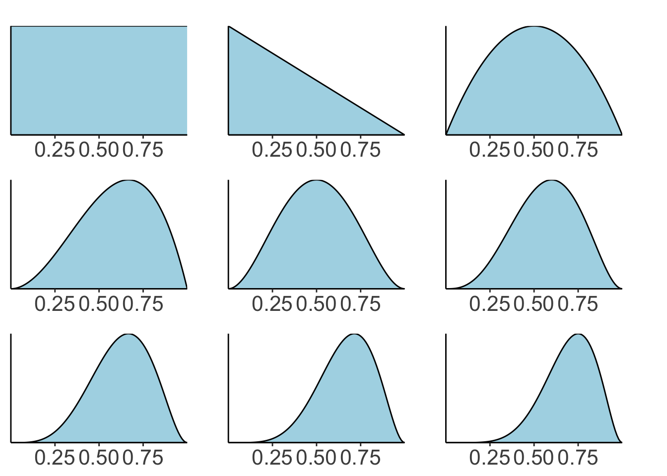
22.3.2 Coin flip example
Is the coin biased?
# data
data = rep(0:1, c(8, 2))

# parameters
theta = c(0.1, 0.5, 0.9)

# prior
prior = c(0.25, 0.5, 0.25)
# prior = c(0.1, 0.1, 0.8) # alternative setting of the prior
# prior = c(0.000001, 0.000001, 0.999998) # another prior setting

# likelihood
likelihood = dbinom(sum(data == 1), size = length(data), prob = theta)

# posterior
posterior = likelihood * prior / sum(likelihood * prior)

# store in data frame
df.coins = tibble(theta = theta,
                  prior = prior,
                  likelihood = likelihood,
                  posterior = posterior)
Visualize the results:
df.coins %>%
  pivot_longer(cols = -theta,
               names_to = "index",
               values_to = "value") %>%
  mutate(index = factor(index, levels = c("prior", "likelihood", "posterior")),
         theta = factor(theta, labels = c("p = 0.1", "p = 0.5", "p = 0.9"))) %>%
  ggplot(data = .,
         mapping = aes(x = theta,
                       y = value,
                       fill = index)) +
  geom_bar(stat = "identity",
           color = "black") +
  facet_grid(rows = vars(index),
             switch = "y",
             scales = "free") +
  annotate("segment", x = -Inf, xend = Inf, y = -Inf, yend = -Inf) +
  annotate("segment", x = -Inf, xend = -Inf, y = -Inf, yend = Inf) +
  theme(legend.position = "none",
        strip.background = element_blank(),
        axis.title.y = element_blank(),
        axis.text.y = element_blank(),
        axis.ticks.y = element_blank(),
        axis.title.x = element_blank(),
        axis.line = element_blank())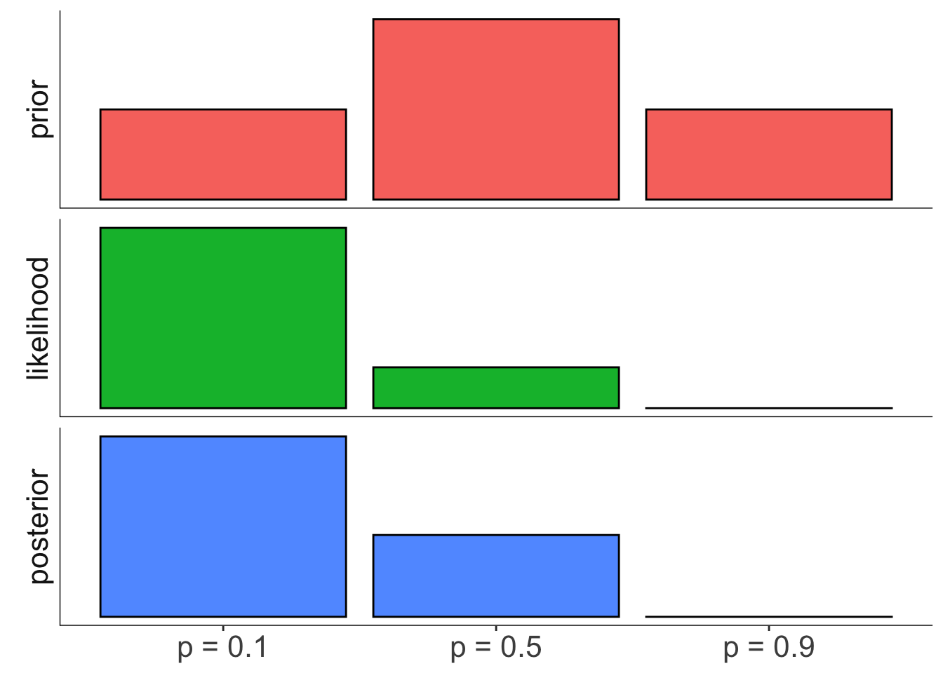
22.3.3 Bayesian inference by discretization
22.3.3.1 Effect of the prior
# grid
theta = seq(0, 1, 0.01)

# data
data = rep(0:1, c(8, 2))

# calculate posterior
df.prior_effect = tibble(theta = theta,
                  prior_uniform = dbeta(theta, shape1 = 1, shape2 = 1),
                  prior_normal = dbeta(theta, shape1 = 5, shape2 = 5),
                  prior_biased = dbeta(theta, shape1 = 8, shape2 = 2)) %>%
  pivot_longer(cols = -theta,
               names_to = "prior_index",
               values_to = "prior") %>%
  mutate(likelihood = dbinom(sum(data == 1),
                             size = length(data),
                             prob = theta)) %>%
  group_by(prior_index) %>%
  mutate(posterior = likelihood * prior / sum(likelihood * prior)) %>%
  ungroup() %>%
  pivot_longer(cols = -c(theta, prior_index),
               names_to = "index",
               values_to = "value")

# make the plot
df.prior_effect %>%
  mutate(index = factor(index, levels = c("prior", "likelihood", "posterior")),
         prior_index = factor(prior_index,
                              levels = c("prior_uniform", "prior_normal", "prior_biased"),
                              labels = c("uniform", "symmetric", "asymmetric"))) %>%
  ggplot(data = .,
         mapping = aes(x = theta,
                       y = value,
                       color = index)) +
  geom_line(size = 1) +
  facet_grid(cols = vars(prior_index),
             rows = vars(index),
             scales = "free",
             switch = "y") +
  scale_x_continuous(breaks = seq(0, 1, 0.2)) +
  annotate("segment", x = -Inf, xend = Inf, y = -Inf, yend = -Inf) +
  annotate("segment", x = -Inf, xend = -Inf, y = -Inf, yend = Inf) +
  theme(legend.position = "none",
        strip.background = element_blank(),
        axis.title.y = element_blank(),
        axis.text.y = element_blank(),
        axis.ticks.y = element_blank(),
        axis.text.x = element_text(size = 10),
        axis.line = element_blank())
Warning: Using `size` aesthetic for lines was deprecated in ggplot2 3.4.0.
ℹ Please use `linewidth` instead.
This warning is displayed once every 8 hours.
Call `lifecycle::last_lifecycle_warnings()` to see where this warning was generated.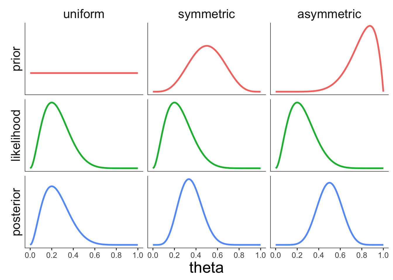
Figure 2.7: Illustration of how the prior affects the posterior.
22.3.3.2 Effect of the likelihood
# grid
theta = seq(0, 1, 0.01)

df.likelihood_effect = tibble(theta = theta,
                              prior = dbeta(theta, shape1 = 2, shape2 = 8),
                              likelihood_left = dbeta(theta, shape1 = 1, shape2 = 9),
                              likelihood_center = dbeta(theta, shape1 = 5, shape2 = 5),
                              likelihood_right = dbeta(theta, shape1 = 9, shape2 = 1)) %>%
  pivot_longer(cols = -c(theta, prior),
               names_to = "likelihood_index",
               values_to = "likelihood") %>%
  group_by(likelihood_index) %>%
  mutate(posterior = likelihood * prior / sum(likelihood * prior)) %>%
  ungroup() %>%
  pivot_longer(cols = -c(theta, likelihood_index),
               names_to = "index",
               values_to = "value")

df.likelihood_effect %>%
  mutate(index = factor(index, levels = c("prior", "likelihood", "posterior")),
         likelihood_index = factor(likelihood_index,
                                   levels = c("likelihood_left",
                                              "likelihood_center",
                                              "likelihood_right"),
                                   labels = c("left", "center", "right"))) %>%
  ggplot(data = .,
         mapping = aes(x = theta,
                       y = value,
                       color = index)) +
  geom_line(size = 1) +
  facet_grid(cols = vars(likelihood_index),
             rows = vars(index),
             scales = "free",
             switch = "y") +
  scale_x_continuous(breaks = seq(0, 1, 0.2)) +
  annotate("segment", x = -Inf, xend = Inf, y = -Inf, yend = -Inf) +
  annotate("segment", x = -Inf, xend = -Inf, y = -Inf, yend = Inf) +
  theme(legend.position = "none",
        strip.background = element_blank(),
        axis.title.y = element_blank(),
        axis.text.y = element_blank(),
        axis.ticks.y = element_blank(),
        axis.text.x = element_text(size = 10),
        axis.line = element_blank(),
        strip.text.x = element_blank())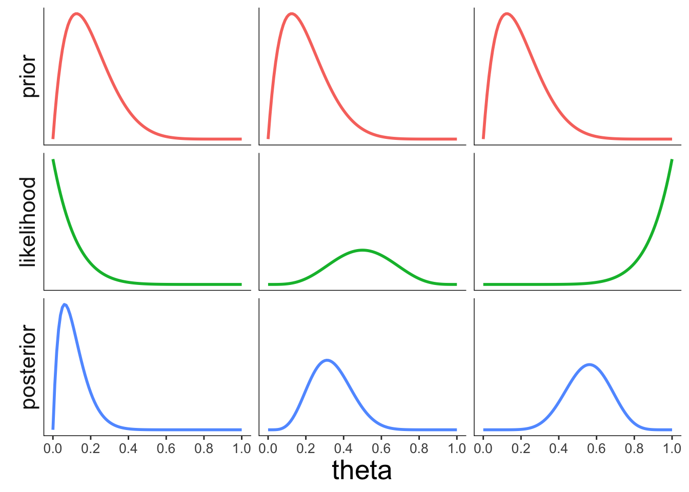
Figure 2.8: Illustration of how the likelihood of the data affects the posterior.
22.3.3.3 Effect of the sample size
# grid
theta = seq(0, 1, 0.01)

df.sample_size_effect = tibble(theta = theta,
                               prior = dbeta(theta, shape1 = 5, shape2 = 5),
                               likelihood_low = dbeta(theta, shape1 = 2, shape2 = 8),
                               likelihood_medium = dbeta(theta,
                                                         shape1 = 10,
                                                         shape2 = 40),
                               likelihood_high = dbeta(theta,
                                                       shape1 = 20,
                                                       shape2 = 80)) %>%
  pivot_longer(cols = -c(theta, prior),
               names_to = "likelihood_index",
               values_to = "likelihood") %>%
  group_by(likelihood_index) %>%
  mutate(posterior = likelihood * prior / sum(likelihood * prior)) %>%
  ungroup() %>%
  pivot_longer(cols = -c(theta, likelihood_index),
               names_to = "index",
               values_to = "value")

df.sample_size_effect %>%
  mutate(index = factor(index, levels = c("prior", "likelihood", "posterior")),
         likelihood_index = factor(likelihood_index,
                                   levels = c("likelihood_low",
                                              "likelihood_medium",
                                              "likelihood_high"),
                                   labels = c("n = low", "n = medium", "n = high"))) %>%
  ggplot(data = .,
         mapping = aes(x = theta,
                       y = value,
                       color = index)) +
  geom_line(size = 1) +
  facet_grid(cols = vars(likelihood_index),
             rows = vars(index),
             scales = "free",
             switch = "y") +
  scale_x_continuous(breaks = seq(0, 1, 0.2)) +
  annotate("segment", x = -Inf, xend = Inf, y = -Inf, yend = -Inf) +
  annotate("segment", x = -Inf, xend = -Inf, y = -Inf, yend = Inf) +
  theme(legend.position = "none",
        strip.background = element_blank(),
        axis.title.y = element_blank(),
        axis.text.y = element_blank(),
        axis.ticks.y = element_blank(),
        axis.text.x = element_text(size = 10),
        axis.line = element_blank())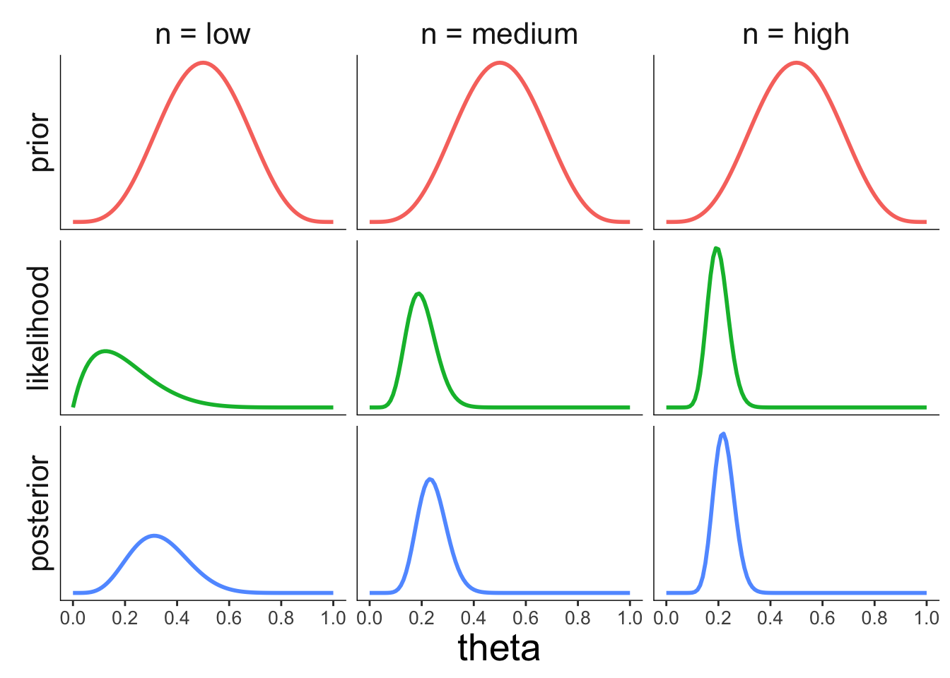
22.4 Doing Bayesian inference with Greta
You can find out more about how get started with “greta” here: https://greta-stats.org/articles/get_started.html. Make sure to install the development version of “greta” (as shown in the “install-packages” code chunk above: devtools::install_github("greta-dev/greta")).
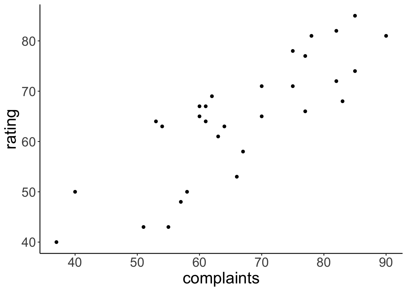
22.4.1 Attitude data set
Visualize relationship between how well complaints are handled and the overall rating of an employee
22.4.2 Frequentist analysis
# fit model
fit.lm = lm(formula = rating ~ 1 + complaints,
            data = df.attitude)

# print summary
fit.lm %>%
  summary()
Call:
lm(formula = rating ~ 1 + complaints, data = df.attitude)

Residuals:
     Min       1Q   Median       3Q      Max
-12.8799  -5.9905   0.1783   6.2978   9.6294

Coefficients:
            Estimate Std. Error t value Pr(>|t|)
(Intercept) 14.37632    6.61999   2.172   0.0385 *
complaints   0.75461    0.09753   7.737 1.99e-08 ***
---
Signif. codes:  0 '***' 0.001 '**' 0.01 '*' 0.05 '.' 0.1 ' ' 1

Residual standard error: 6.993 on 28 degrees of freedom
Multiple R-squared:  0.6813,    Adjusted R-squared:  0.6699
F-statistic: 59.86 on 1 and 28 DF,  p-value: 1.988e-08
Visualize the model’s predictions
ggplot(data = df.attitude,
       mapping = aes(x = complaints,
                     y = rating)) +
  geom_smooth(method = "lm",
              formula = "y ~ x",
              color = "black") +
  geom_point()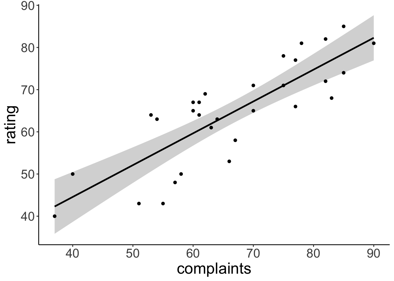
22.4.3 Bayesian regression
22.4.3.1 Fit the model
set.seed(1)

# variables & priors
b0 = normal(0, 10)
b1 = normal(0, 10)
sd = cauchy(0, 3, truncation = c(0, Inf))

# linear predictor
mu = b0 + b1 * df.attitude$complaints

# observation model (likelihood)
distribution(df.attitude$rating) = normal(mu, sd)

# define the model
m = model(b0, b1, sd)
Visualize the model as graph:
Draw samples from the posterior distribution:
22.4.3.2 Visualize the priors
These are the priors I used for the intercept, regression weights, and the standard deviation of the Gaussian likelihood function:
22.4.3.3 Visualize the posteriors
This is what the posterior looks like for the three parameters in the model:
df.draws %>%
  select(draw:sd) %>%
  pivot_longer(cols = -draw,
               names_to = "index",
               values_to = "value") %>%
  ggplot(data = .,
         mapping = aes(x = value)) +
  stat_density(geom = "line") +
  facet_grid(rows = vars(index),
             scales = "free_y",
             switch = "y") +
  annotate("segment", x = -Inf, xend = Inf, y = -Inf, yend = -Inf) +
  annotate("segment", x = -Inf, xend = -Inf, y = -Inf, yend = Inf) +
  theme(legend.position = "none",
        strip.background = element_blank(),
        axis.title.y = element_blank(),
        axis.text.y = element_blank(),
        axis.ticks.y = element_blank(),
        axis.text.x = element_text(size = 10),
        axis.line = element_blank(),
strip.text.x = element_blank())22.4.3.5 Visualize model predictions
Let’s take some samples from the posterior to visualize the model predictions:
22.4.3.6 Posterior predictive check
Let’s make an animation that illustrates what predicted data sets (based on samples from the posterior) would look like:
p = df.draws %>%
  slice_sample(n = 10) %>%
  mutate(complaints = list(seq(min(df.attitude$complaints),
                               max(df.attitude$complaints),
                               length.out = nrow(df.attitude)))) %>%
  unnest(c(complaints)) %>%
  mutate(prediction = b0 + b1 * complaints + rnorm(n(), sd = sd)) %>%
  ggplot(aes(x = complaints, y = prediction)) +
  geom_point(alpha = 0.8,
             color = "lightblue") +
  geom_point(data = df.attitude,
             aes(y = rating,
                 x = complaints)) +
  coord_cartesian(xlim = c(20, 100),
                  ylim = c(20, 100)) +
  transition_manual(draw)

animate(p,
        nframes = 60,
        width = 800,
        height = 600,
        res = 96,
        type = "cairo")

# anim_save("posterior_predictive.gif")
22.4.3.7 Prior predictive check
And let’s illustrate what data we would have expected to see just based on the information that we encoded in our priors.
sample_size = 10

p = tibble(b0 = rnorm(sample_size, mean = 0, sd = 10),
           b1 = rnorm(sample_size, mean = 0, sd = 10),
           sd = rhcauchy(sample_size, sigma = 3),
           draw = 1:sample_size) %>%
  mutate(complaints = list(runif(nrow(df.attitude),
                                 min = min(df.attitude$complaints),
                                 max = max(df.attitude$complaints)))) %>%
  unnest(c(complaints)) %>%
  mutate(prediction = b0 + b1 * complaints + rnorm(n(), sd = sd)) %>%
  ggplot(aes(x = complaints, y = prediction)) +
  geom_point(alpha = 0.8,
             color = "lightblue") +
  geom_point(data = df.attitude,
             aes(y = rating,
                 x = complaints)) +
  transition_manual(draw)

animate(p,
        nframes = 60,
        width = 800,
        height = 600,
        res = 96,
        type = "cairo")

# anim_save("prior_predictive.gif")22.6 Session info
Information about this R session including which version of R was used, and what packages were loaded.
R version 4.4.2 (2024-10-31)
Platform: aarch64-apple-darwin20
Running under: macOS Sequoia 15.2

Matrix products: default
BLAS:   /Library/Frameworks/R.framework/Versions/4.4-arm64/Resources/lib/libRblas.0.dylib
LAPACK: /Library/Frameworks/R.framework/Versions/4.4-arm64/Resources/lib/libRlapack.dylib;  LAPACK version 3.12.0

locale:
[1] en_US.UTF-8/en_US.UTF-8/en_US.UTF-8/C/en_US.UTF-8/en_US.UTF-8

time zone: America/Los_Angeles
tzcode source: internal

attached base packages:
[1] stats     graphics  grDevices utils     datasets  methods   base

other attached packages:
 [1] lubridate_1.9.3   forcats_1.0.0     stringr_1.5.1     dplyr_1.1.4
 [5] purrr_1.0.2       readr_2.1.5       tidyr_1.3.1       tibble_3.2.1
 [9] tidyverse_2.0.0   broom_1.0.7       extraDistr_1.10.0 gganimate_1.0.9
[13] ggplot2_3.5.1     greta_0.5.0       tidybayes_3.0.7   patchwork_1.3.0
[17] janitor_2.2.1     knitr_1.49

loaded via a namespace (and not attached):
 [1] svUnit_1.0.6         tidyselect_1.2.1     farver_2.1.2
 [4] tensorflow_2.16.0    fastmap_1.2.0        tensorA_0.36.2.1
 [7] tweenr_2.0.3         digest_0.6.36        timechange_0.3.0
[10] lifecycle_1.0.4      processx_3.8.4       magrittr_2.0.3
[13] posterior_1.6.0      compiler_4.4.2       rlang_1.1.4
[16] sass_0.4.9           progress_1.2.3       tools_4.4.2
[19] utf8_1.2.4           yaml_2.3.10          labeling_0.4.3
[22] prettyunits_1.2.0    reticulate_1.38.0    abind_1.4-5
[25] withr_3.0.2          grid_4.4.2           fansi_1.0.6
[28] colorspace_2.1-0     future_1.33.2        globals_0.16.3
[31] scales_1.3.0         cli_3.6.3            rmarkdown_2.29
[34] crayon_1.5.3         generics_0.1.3       tzdb_0.4.0
[37] tfruns_1.5.3         cachem_1.1.0         splines_4.4.2
[40] parallel_4.4.2       base64enc_0.1-3      vctrs_0.6.5
[43] Matrix_1.7-1         jsonlite_1.8.8       bookdown_0.42
[46] callr_3.7.6          hms_1.1.3            arrayhelpers_1.1-0
[49] listenv_0.9.1        ggdist_3.3.2         jquerylib_0.1.4
[52] glue_1.8.0           parallelly_1.37.1    codetools_0.2-20
[55] ps_1.7.7             distributional_0.4.0 stringi_1.8.4
[58] gtable_0.3.5         munsell_0.5.1        pillar_1.9.0
[61] htmltools_0.5.8.1    R6_2.5.1             evaluate_0.24.0
[64] lattice_0.22-6       png_0.1-8            backports_1.5.0
[67] snakecase_0.11.1     bslib_0.7.0          Rcpp_1.0.13
[70] nlme_3.1-166         coda_0.19-4.1        checkmate_2.3.1
[73] mgcv_1.9-1           whisker_0.4.1        xfun_0.49
[76] pkgconfig_2.0.3