Chapter 6 Probability

6.1 Load packages, load data, set theme

Let’s load the packages that we need for this chapter.

library("knitr")        # for rendering the RMarkdown file
library("kableExtra")   # for nicely formatted tables
library("arrangements") # fast generators and iterators for creating combinations
library("DiagrammeR")   # for drawing diagrams
library("tidyverse")    # for data wrangling 

Set the plotting theme.

theme_set(theme_classic() + 
            theme(text = element_text(size = 20)))

opts_chunk$set(comment = "",
               fig.show = "hold")

6.2 Counting

Imagine that there are three balls in an urn. The balls are labeled 1, 2, and 3. Let’s consider a few possible situations.

balls = 1:3 # number of balls in urn 
ndraws = 2 # number of draws

# order matters, without replacement
permutations(balls, ndraws)

     [,1] [,2]
[1,]    1    2
[2,]    1    3
[3,]    2    1
[4,]    2    3
[5,]    3    1
[6,]    3    2

# order matters, with replacement
permutations(balls, ndraws, replace = T)

      [,1] [,2]
 [1,]    1    1
 [2,]    1    2
 [3,]    1    3
 [4,]    2    1
 [5,]    2    2
 [6,]    2    3
 [7,]    3    1
 [8,]    3    2
 [9,]    3    3

# order doesn't matter, with replacement 
combinations(balls, ndraws, replace = T)

     [,1] [,2]
[1,]    1    1
[2,]    1    2
[3,]    1    3
[4,]    2    2
[5,]    2    3
[6,]    3    3

# order doesn't matter, without replacement 
combinations(balls, ndraws)

     [,1] [,2]
[1,]    1    2
[2,]    1    3
[3,]    2    3

I’ve generated the figures below using the DiagrammeR package. It’s a powerful package for drawing diagrams in R. See information on how to use the DiagrammeR package here.

Figure 6.1: Drawing two marbles out of an urn with replacement.

Figure 6.2: Drawing two marbles out of an urn without replacement.

6.3 The random secretary

A secretary types four letters to four people and addresses the four envelopes. If he inserts the letters at random, each in a different envelope, what is the probability that exactly three letters will go into the right envelope?

df.letters = permutations(x = 1:4, k = 4) %>% 
  as_tibble(.name_repair = ~ str_c("person_", 1:4)) %>%
  mutate(n_correct = (person_1 == 1) + 
           (person_2 == 2) + 
           (person_3 == 3) +
           (person_4 == 4))

df.letters %>% 
  summarize(prob_3_correct = sum(n_correct == 3) / n())

# A tibble: 1 × 1
  prob_3_correct
           <dbl>
1              0

ggplot(data = df.letters,
       mapping = aes(x = n_correct)) + 
  geom_bar(aes(y = stat(count)/sum(count)),
           color = "black",
           fill = "lightblue") +
  scale_y_continuous(labels = scales::percent,
                     expand = c(0, 0)) + 
  labs(x = "number correct",
       y = "probability")

Warning: `stat(count)` was deprecated in ggplot2 3.4.0.
ℹ Please use `after_stat(count)` instead.
This warning is displayed once every 8 hours.
Call `lifecycle::last_lifecycle_warnings()` to see where this warning was
generated.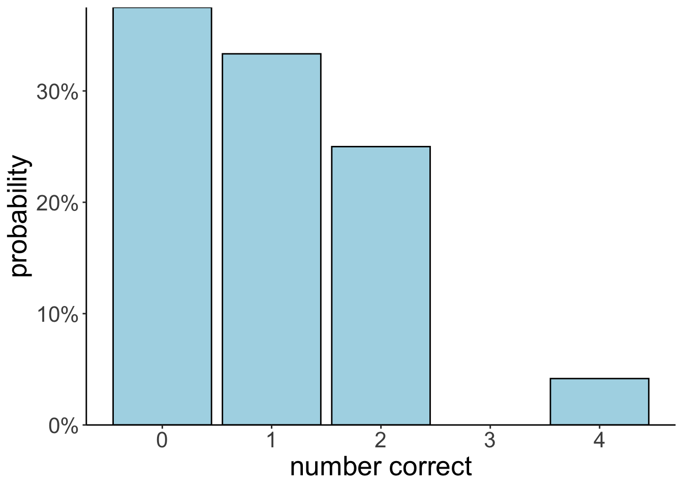

6.4 Flipping a coin many times

# Example taken from here: http://statsthinking21.org/probability.html#empirical-frequency

set.seed(1) # set the seed so that the outcome is consistent
nsamples = 50000 # how many flips do we want to make?

# create some random coin flips using the rbinom() function with
# a true probability of 0.5

df.samples = tibble(trial_number = seq(nsamples), 
                    outcomes = rbinom(nsamples, 1, 0.5)) %>% 
  mutate(mean_probability = cumsum(outcomes) / seq_along(outcomes)) %>% 
  filter(trial_number >= 10) # start with a minimum sample of 10 flips

ggplot(data = df.samples, 
       mapping = aes(x = trial_number, y = mean_probability)) +
  geom_hline(yintercept = 0.5, color = "gray", linetype = "dashed") +
  geom_line() +
  labs(x = "Number of trials",
       y = "Estimated probability of heads") +
  theme_classic() +
  theme(text = element_text(size = 20))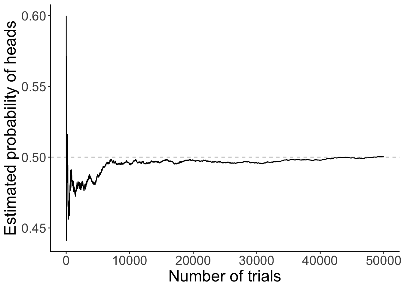

Figure 6.3: A demonstration of the law of large numbers.

6.5 Clue guide to probability

who = c("ms_scarlet", "col_mustard", "mrs_white",
        "mr_green", "mrs_peacock", "prof_plum")
what = c("candlestick", "knife", "lead_pipe",
         "revolver", "rope", "wrench")
where = c("study", "kitchen", "conservatory",
          "lounge", "billiard_room", "hall",
          "dining_room", "ballroom", "library")

df.clue = expand_grid(who = who,
                      what = what,
                      where = where)

df.suspects = df.clue %>% 
  distinct(who) %>% 
  mutate(gender = ifelse(test = who %in% c("ms_scarlet", "mrs_white", "mrs_peacock"), 
                         yes = "female", 
                         no = "male"))

df.suspects %>% 
  arrange(desc(gender)) %>% 
  kable() %>% 
  kable_styling("striped", full_width = F)

who	gender
col_mustard	male
mr_green	male
prof_plum	male
ms_scarlet	female
mrs_white	female
mrs_peacock	female

6.5.1 Conditional probability

# conditional probability (via rules of probability)
df.suspects %>% 
  summarize(p_prof_plum_given_male = 
              sum(gender == "male" & who == "prof_plum") /
              sum(gender == "male"))

# A tibble: 1 × 1
  p_prof_plum_given_male
                   <dbl>
1                  0.333

# conditional probability (via rejection)
df.suspects %>% 
  filter(gender == "male") %>% 
  summarize(p_prof_plum_given_male = 
              sum(who == "prof_plum") /
              n())

# A tibble: 1 × 1
  p_prof_plum_given_male
                   <dbl>
1                  0.333

6.5.2 Law of total probability

6.6 Probability operations

# Make a deck of cards 
df.cards = tibble(suit = rep(c("Clubs", "Spades", "Hearts", "Diamonds"), each = 8),
                  value = rep(c("7", "8", "9", "10", "Jack", "Queen", "King", "Ace"), 4)) 

# conditional probability: p(Hearts | Queen) (via rules of probability)
df.cards %>% 
  summarize(p_hearts_given_queen = 
              sum(suit == "Hearts" & value == "Queen") / 
              sum(value == "Queen"))

# A tibble: 1 × 1
  p_hearts_given_queen
                 <dbl>
1                 0.25

# conditional probability: p(Hearts | Queen) (via rejection)
df.cards %>% 
  filter(value == "Queen") %>%
  summarize(p_hearts_given_queen = sum(suit == "Hearts")/n())

# A tibble: 1 × 1
  p_hearts_given_queen
                 <dbl>
1                 0.25

6.7 Bayesian reasoning explained

6.8 Getting Bayes right matters

6.8.1 Bayesian reasoning example

# prior probability of the disease
p.D = 0.0001

# sensitivity of the test 
p.T_given_D = 0.999

# specificity of the test 
p.notT_given_notD = 0.999
p.T_given_notD = (1 - p.notT_given_notD)

# posterior given a positive test result 
p.D_given_T = (p.T_given_D * p.D) / ((p.T_given_D * p.D) + (p.T_given_notD * (1-p.D)))

p.D_given_T

[1] 0.0908347

6.8.2 Bayesian reasoning example (COVID rapid test)

https://pubmed.ncbi.nlm.nih.gov/34242764/#:~:text=The%20overall%20sensitivity%20of%20the,%25%20CI%2024.4%2D65.1).

# prior probability of the disease
p.D = 0.1 

# sensitivity covid rapid test
p.T_given_D = 0.653

# specificity of covid rapid test
p.notT_given_notD = 0.999

p.T_given_notD = (1 - p.notT_given_notD)

# posterior given a positive test result 
p.D_given_T = (p.T_given_D * p.D) / ((p.T_given_D * p.D) + (p.T_given_notD * (1-p.D)))

# posterior given a negative test result 
p.D_given_notT = ((1-p.T_given_D) * p.D) / (((1-p.T_given_D) * p.D) + ((1-p.T_given_notD) * (1-p.D)))

str_c("Probability of COVID given a positive test: ", round(p.D_given_T * 100, 1), "%")

[1] "Probability of COVID given a positive test: 98.6%"

str_c("Probability of COVID given a negative test: ", round(p.D_given_notT * 100, 1), "%")

[1] "Probability of COVID given a negative test: 3.7%"

6.8.3 Most people in the hospital are vaccinated

# probability of being vaccinated 
p.V = 0.8 

# likelihood of hospital 
p.H_given_V = 0.2
p.H_given_notV = 0.5

# posterior probability 
p.V_given_H = (p.H_given_V * p.V) / ((p.H_given_V * p.V) + (p.H_given_notV * (1-p.V)))

p.V_given_H

[1] 0.6153846

6.9 Building a Bayesis

6.9.1 Dice example

# prior
p.four = 0.5
p.six = 0.5

# possibilities 
df.possibilities = tibble(observation = 1:6,
                          p.four = c(rep(1/4, 4), rep(0, 2)),
                          p.six = c(rep(1/6, 6)))

# data
# data = c(4)
# data = c(4, 2, 1)
data = c(4, 2, 1, 3, 1)
# data = c(4, 2, 1, 3, 1, 5)

# likelihood
p.data_given_four = prod(df.possibilities$p.four[data])
p.data_given_six = prod(df.possibilities$p.six[data])

# posterior
p.four_given_data = (p.data_given_four * p.four) /  
  ((p.data_given_four * p.four) + 
     (p.data_given_six * p.six))

p.four_given_data

[1] 0.8836364

Given this data \(d\) = [4, 2, 1, 3, 1], there is a 88% chance that the four sided die was rolled rather than the six sided die.

6.10 Additional resources

6.10.1 Cheatsheets

• Probability cheatsheet

6.10.2 Books and chapters

• Probability and Statistics with examples using R
• Learning statistics with R: Chapter 9 Introduction to probability

6.10.3 Misc

• Bayes’ theorem in three panels
• Statistics 110: Probability; course at Harvard
  
• Bayes theorem and making probability intuitive

6.11 Session info

Information about this R session including which version of R was used, and what packages were loaded.

R version 4.3.2 (2023-10-31)
Platform: aarch64-apple-darwin20 (64-bit)
Running under: macOS Sonoma 14.1.2

Matrix products: default
BLAS:   /Library/Frameworks/R.framework/Versions/4.3-arm64/Resources/lib/libRblas.0.dylib 
LAPACK: /Library/Frameworks/R.framework/Versions/4.3-arm64/Resources/lib/libRlapack.dylib;  LAPACK version 3.11.0

locale:
[1] en_US.UTF-8/en_US.UTF-8/en_US.UTF-8/C/en_US.UTF-8/en_US.UTF-8

time zone: America/Los_Angeles
tzcode source: internal

attached base packages:
[1] stats     graphics  grDevices utils     datasets  methods   base     

other attached packages:
 [1] lubridate_1.9.3    forcats_1.0.0      stringr_1.5.1      dplyr_1.1.4       
 [5] purrr_1.0.2        readr_2.1.4        tidyr_1.3.0        tibble_3.2.1      
 [9] ggplot2_3.4.4      tidyverse_2.0.0    DiagrammeR_1.0.10  arrangements_1.1.9
[13] kableExtra_1.3.4   knitr_1.45        

loaded via a namespace (and not attached):
 [1] gmp_0.7-3          sass_0.4.8         utf8_1.2.4         generics_0.1.3    
 [5] xml2_1.3.6         stringi_1.8.3      hms_1.1.3          digest_0.6.33     
 [9] magrittr_2.0.3     timechange_0.2.0   evaluate_0.23      grid_4.3.2        
[13] RColorBrewer_1.1-3 bookdown_0.37      fastmap_1.1.1      jsonlite_1.8.8    
[17] httr_1.4.7         rvest_1.0.3        fansi_1.0.6        viridisLite_0.4.2 
[21] scales_1.3.0       jquerylib_0.1.4    cli_3.6.2          crayon_1.5.2      
[25] rlang_1.1.2        visNetwork_2.1.2   ellipsis_0.3.2     munsell_0.5.0     
[29] withr_2.5.2        cachem_1.0.8       yaml_2.3.8         tools_4.3.2       
[33] tzdb_0.4.0         colorspace_2.1-0   webshot_0.5.5      vctrs_0.6.5       
[37] R6_2.5.1           lifecycle_1.0.4    htmlwidgets_1.6.4  pkgconfig_2.0.3   
[41] bslib_0.6.1        pillar_1.9.0       gtable_0.3.4       glue_1.6.2        
[45] systemfonts_1.0.5  highr_0.10         xfun_0.41          tidyselect_1.2.0  
[49] rstudioapi_0.15.0  farver_2.1.1       htmltools_0.5.7    labeling_0.4.3    
[53] rmarkdown_2.25     svglite_2.1.3      compiler_4.3.2